Understanding the Benjamini–Hochberg procedure

Last updated on Mar 20, 2021 6 min read

The prnSig and pepSig utilities in proteoQ perform significance analysis for protein and peptide data, respectively. In what follows the step of p-value assessment, multiple test corrections using the stats::p.adjust will be carried out, with the Benjamini–Hochberg (BH) procedure being the default.

Occasionally, we may run into situations where a handful of adjusted p-values equal one with near perfection. These large p-values are insignificant and uninteresting, however annoying, if without a clear elucidation of the probable causes to researchers. For this reason, I would take a break to find out the intuition behind the BH procedure.

Hypothesis testing and false discovery rate

In statistical theory, a hypothesis testing problem is about the decision between two competing statements: the null hypothesis, \(H_0\), and the alternative hypothesis, \(H_1\). A null hypothesis may be a statement such that “a perturbation on average has no effect on the expression of a gene” and an alternative is the complement.

A test of \(H_0\) versus \(H_1\) might make one of the two types of errors: Type I error (false positive) and Type II error (false negative). The overall findings following a number of tests, \(H_{0i}\) versus \(H_{1i}\) where \(i = 1, 2, \cdots, m\), are often tabularized in the following format or alike:

Hypothesis	Number of \(H_0\) accepted	Number of \(H_1\) accepted	Total
\(H_0\)	\(\mathbf{U}\)	\(\mathbf{V}\)	\(m_0\)
\(H_1\)	\(\mathbf{T}\)	\(\mathbf{S}\)	\(m - m_0\)
	\(m - \mathbf{R}\)	\(\mathbf{R}\)	\(m\)

where

\(m\), the total number hypotheses tested
\(m_{0}\), the number of true null hypotheses
\(m - m_0\), the number of true alternative hypotheses
\(\mathbf{U}\), the number of true negatives (TN)
\(\mathbf{V}\), the number of false positives (FP)
\(\mathbf{T}\), the number of false negatives (FN)
\(\mathbf{S}\), the number of true positives (TP)
\(\mathbf{R=V+S}\), the number of rejected null hypotheses (discoveries)

with the quantities that are directly observable from experiments in red.

False discovery rate (FDR) is then defined as the expected proportion of \(H_0\) that are incorrectly rejected as \(H_1\).

\[ \mathrm{FDR} = \mathbb{E} \left [ \frac{\mathbf{V}}{\mathbf{R}} \right ] \]

The \(\mathrm{FDR}\) concept was formally described by Yoav Benjamini and Yosef Hochberg in 1995 and the corresponding procedure in controlling \(\mathrm{FDR}\) is commonly known as a BH procedure.

Null hypothesis and p-values

Before involving the intuition of the BH procedure, we will digress for a moment and re-familiarize ourselves with some properties of p-values. We first recall that, for true null hypotheses, the probability mass function (pmf) of p-values follows a \(U(0,1)\) distribution (George Casella 2002, ch.8):

\[Pr(p|H_0 = \mathrm{TRUE}) \sim U(0,1)\]

This is to say that, given (“|”) the null hypothesis is true, the random variable of p-values (\(p\)) is uniformly distributed between 0 and 1.¹ The property allows us to abuse a little the notation between p-values and the level of Type I error, \(\alpha\). Namely, at a p-value of 0.01, the \(\alpha\) error is also 0.01 etc. (see George Casella (2002), ch.8 for a more accurate description).

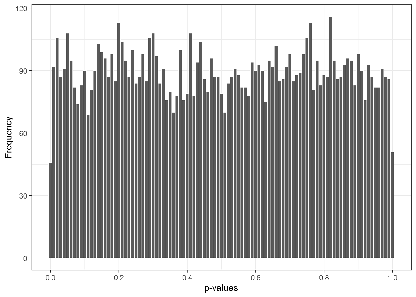
To check the veracity of the theorem, we will generate two sets of simulated \(N(0,1)\) data, each containing 10,000 entries and 20 samples, with 10% of the entries in the second set being offset by \(\pm1\). The p-values are then obtained from two-sample t-tests.

As a first attack, we will temporarily forget the \(H_1\) subset and observe that p-values follow approximately a \(U(0, 1)\) for the \(H_0\) subset.

Recall that the total number of negatives in the \(H_0\) subset is \(m_0\). Thus, the expected number of p-values in the range of \((0, p)\) is \(m_0 p\). We may rephrase the concept in term of Type I error: at a given level of Type I error, \(\alpha\), the expected number of false positives, \(\mathbb{E}(\mathbf{V})\), is \(m_0 \alpha\). For instance with our simulated data, we expect \(9000 \times 0.05\) false positives at the level of \(\alpha = 0.05\) and \(9000 \times 0.01\) at \(\alpha = 0.01\), etc. In other words, we can evaluate \(\mathbb{E}(\mathbf{V})\) at any level \(\alpha\) if \(m_0\) is a known.

Controlling FDR

We now add back the alternative subset, \(H_1\).

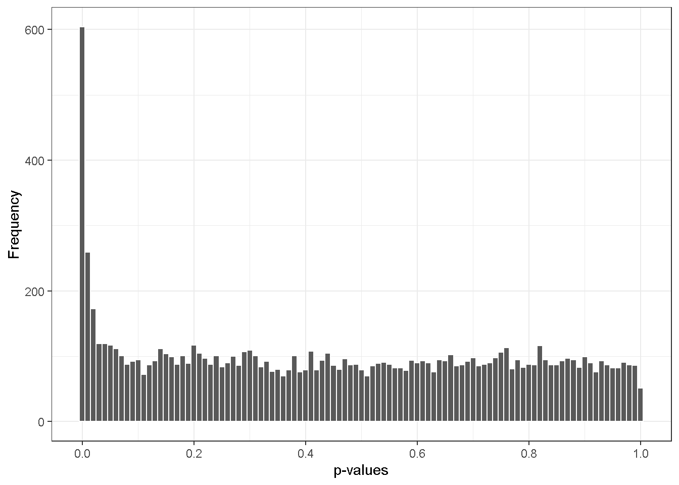
The distribution of p-values is no longer a \(U(0,1)\) because it comprises findings from both the \(H_0\) subset and the \(H_1\) subset. Denote \(r\) the number of hypotheses rejected at the level of \({\alpha}'\) and note that the expected number of false discoveries at the level is \(m_0{\alpha}'\) , we have

\[ \begin{align} \mathrm{FDR} &= \mathbb{E} \left [ \frac{\mathbf{V}}{\mathbf{R}} \right ] \\ &\approx \frac{\mathbb{E}\left[ \mathbf{V} \right]}{\mathbb{E}\left[ \mathbf{R} \right]} \\ &= \frac{m_0{\alpha}'}{r} && (r \text{ is a realization of } \mathbb{E}\left[ \mathbf{R} \right]) \\ &\le \frac{m{\alpha}'}{r} && (m _0 \le m) \\ \end{align} \]

If we can find an \({\alpha}'\) such that \(\frac{m\alpha'}{r} = \alpha\), then the \(\mathrm{FDR}\) is controlled (\(\le \alpha\)).

Adjusted p-value

Finding the level \({\alpha}'\) (p-value) is straightforward. We first rearrange \(\frac{m\alpha'}{r} = \alpha\) to

\[ \begin{align} r = \frac{m}{\alpha}{\alpha}' && (1) \\ \end{align} \]

This corresponds to a line through the origin at a slope of \(m/\alpha\) (the red line; note that we know \(m\) and we choose a starting \(\alpha\)).

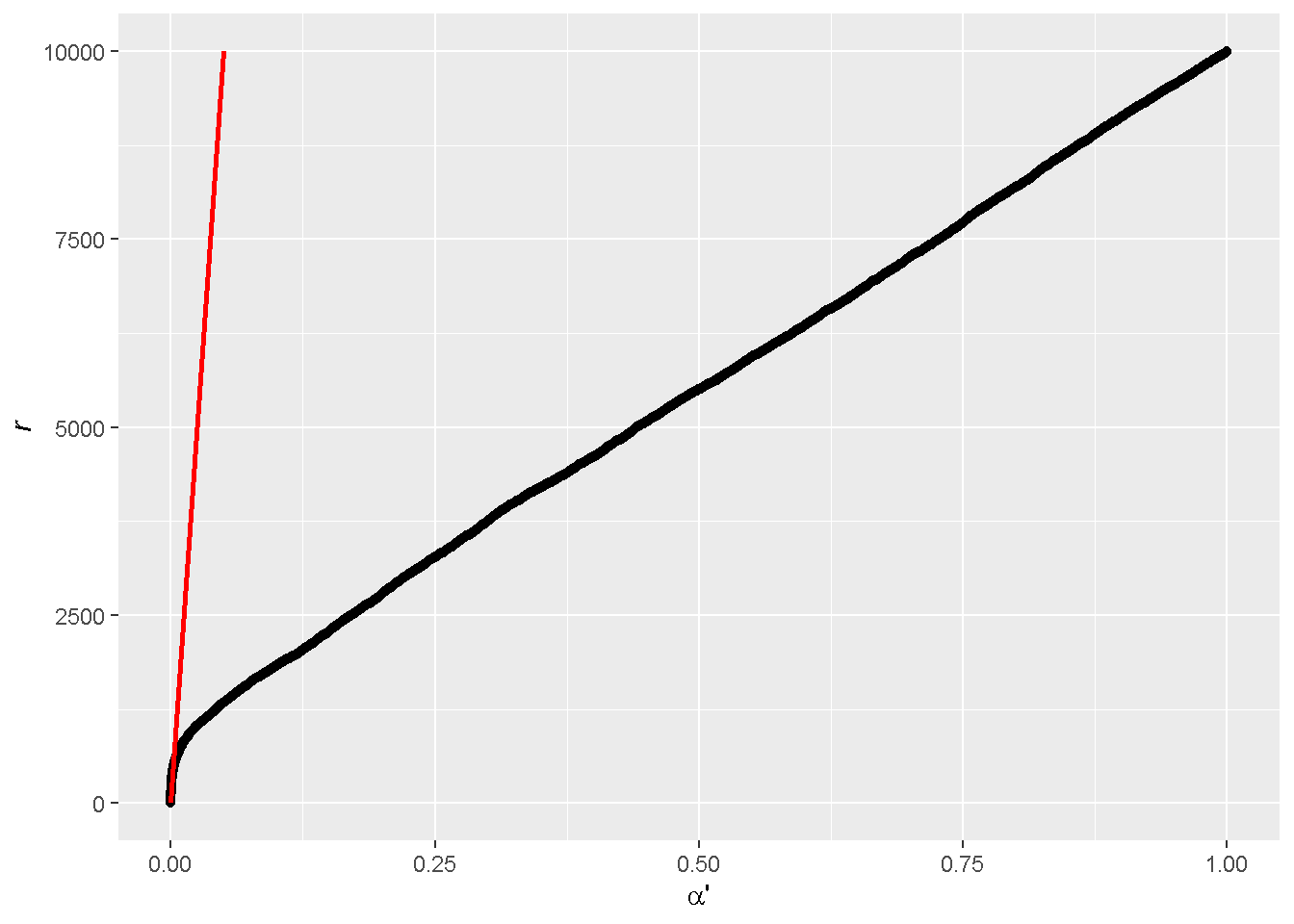
We next order the observed p-values from low to high (the black curve). This allows us to count conveniently the realized number of \(r\) , which is indicated as a coordinate on the y-axis, at a given \({\alpha}'\).

The cross point between the two curves is where the number of rejected null hypotheses measured by experiments (the black curve) agrees with the number budgeted by Eq. 1 (the red line). If we were to move further down in \({\alpha}'\), we would have some unnecessary surplus compared to the budget. That is, the experimentally observed number of \(r\)’s is greater than the needed number of \(r\)’s to satisfy an \(\mathrm{FDR}\) control.

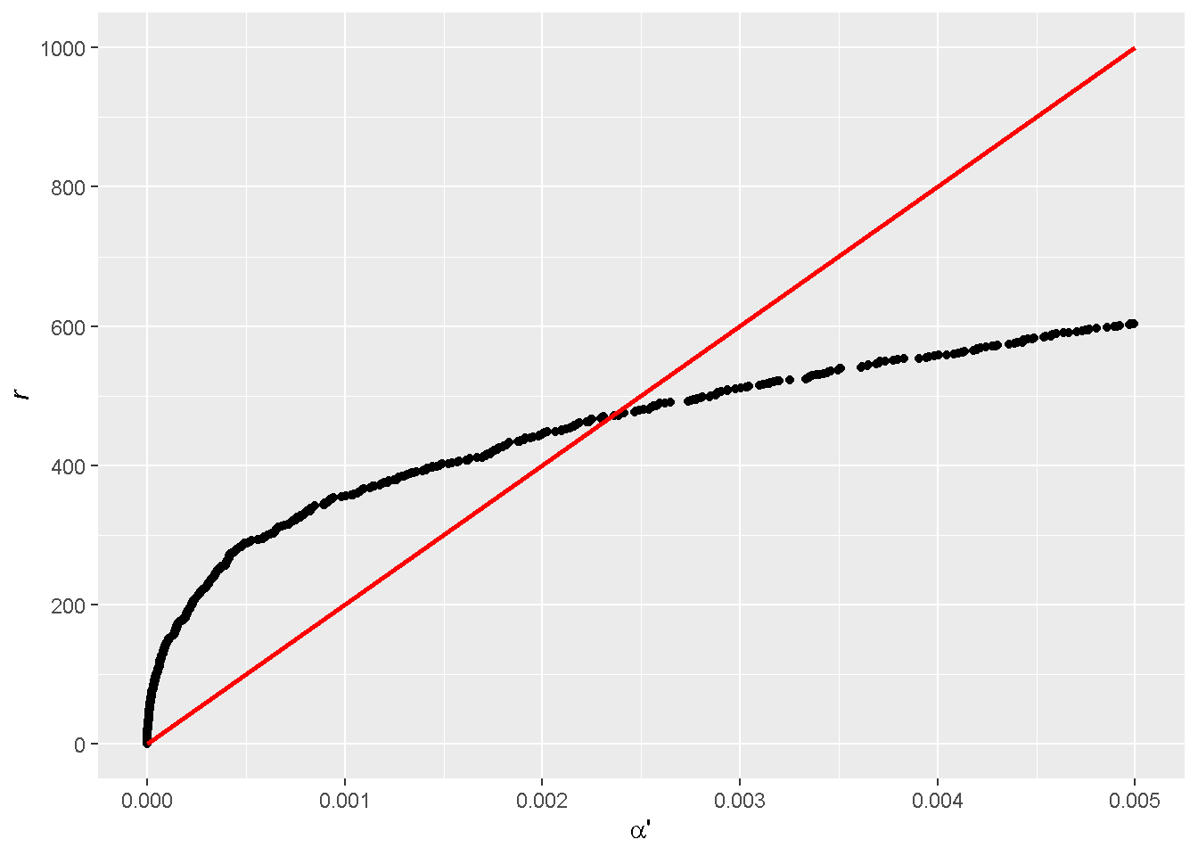
To see the crossing point more closely, we expand the low \({\alpha}'\) region. Recall that the target (adjusted) \(\alpha\) is part of the slope of the red line (Eq. 1), which was actually set to 0.05 in the demonstration! So starting from a goal of \(\alpha = 0.05\) in \(\mathrm{FDR}\) controlling, we end up with an unadjusted \({\alpha}'\) of 0.0024.

By doing the same for different values of \(\alpha\), we can establish the correspondence between adjusted \(\alpha\) and unadjusted \({\alpha}'\).

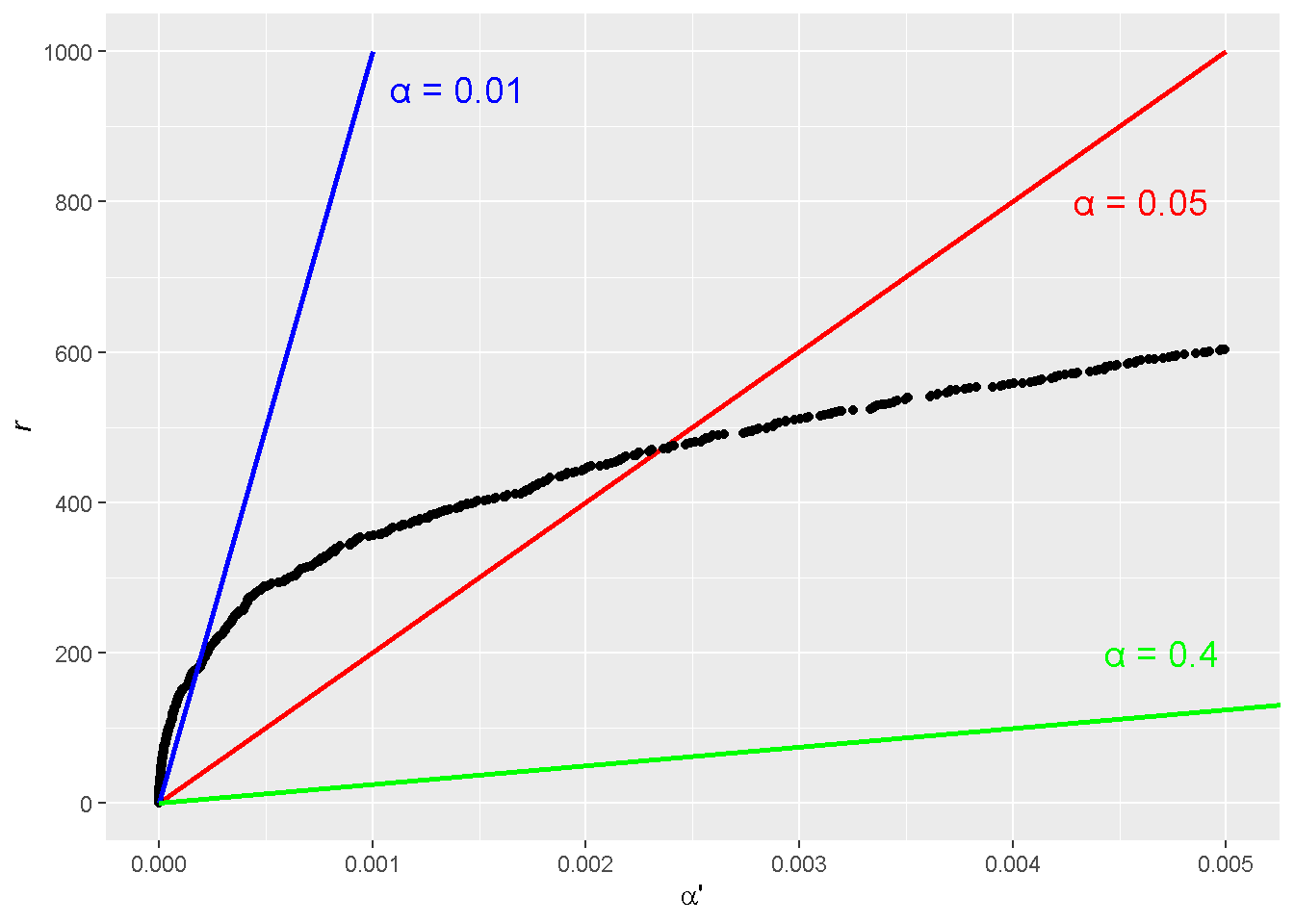
Note that if the slope \(m/\alpha\) is sufficiently small, the budget line might not cut through the black curve of sorted p-values other than the origin. This addresses the question that was raised at the beginning of the post.

References

George Casella, Roger L Berger. 2002. Statistical Inference.

More accurately, the distribution is bound by “\(\le\)” (see the Exercises problem 2.10 in George Casella and Roger Berger, Statistical Inference, 2002). The inequality approaches equality as the distribution of discrete p-values becomes closer and closer to a continuous function.↩︎