LDA in proteoQ

LDA versus PCA

Analogous to the technique of principal component analysis (PCA), LDA involves data projection and abstraction through lines in a high-dimension space. Under a given criterion, it later takes the projections from the dimensions that inform most of the original data cloud for visualization in a low-dimension space.

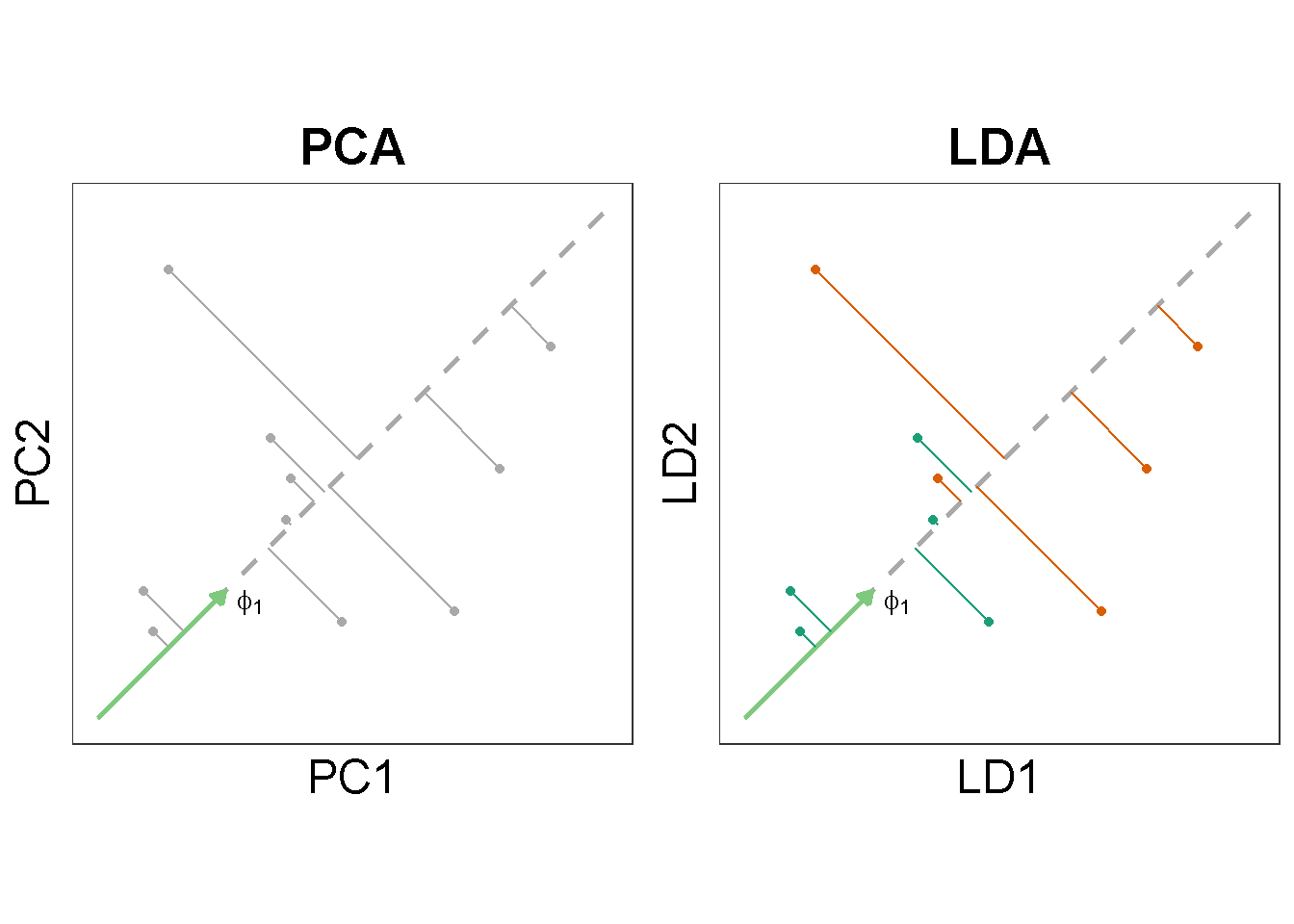
Unlike PCA, the dimensionality reduction by LDA is supervised. In words, LDA makes use of both the expression data \(\mathbf{x}_1, \mathbf{x}_2, \cdots \mathbf{x}_n\) and the associated response \(\y = (y_{1}, y_{2}, \cdots y_{n})\) for the \(n\)-number samples whereas PCA does not involve \(\y\). What does this mean?

Quantities for PCA maximization

In an earlier post, I tried to understand the data projection and variance maximization with basic PCA. Briefly, PCA at first seeks a unit vector, \(\phat\), that corresponds to the greatest sample variance upon projection. In algebraic terms, finding the first principal component is equivalent to maximizing the quantity \(\left \| \X \pone \right \|^{2}\):

\[ \begin{align} \phat &= \argmaxphii \left \| \X \pone \right \|^{2} \\ &= \argmaxphii(\ponet \Xt \X \pone) && \color{blue}{(\text{denote } \A =\Xt \X)} \\ &= \argmaxphii(\ponet \A \pone) && \text{(1)} \\ \end{align} \]

where the variable \(\pone \in \mathbb{R}^p\) is a unit vector and \(\X \in \mathbb{R}^{n \times p}\) is the matrix of expression data with \(n\) samples and \(p\) features. Matrix \(\A = \Xt\X\) is also known as the covariance matrix. Note that PCA takes the data \(\X\) but make no use of the associative category information of the \(n\) samples, should they be available or not.

Quantities for LDA maximization

While PCA maximizes the \(n\)-sample variances as a whole, LDA maximizes the between-class variance relative to the within-class variance (Fisher’s view):

\[ \begin{align} \phat &= \argmaxphii \frac{\ponet \B \pone}{\ponet \W \pone} && \text{(2)} \\ \end{align} \]

where \(\B\) is the between-class covariance and \(\W\) the within-class covariance (Trevor Hastie 2009, Section 4.3.3).¹ Note that in order to calculate \(\B\) and \(\W\), we would subdivide the \(n\) samples by their ascribing groups (see also the previous figure).

Examples with proteoQ

The prnLDA and pepLDA utilities in proteoQ perform the reduced-rank (or dimension) LDA for protein and peptide data, respectively. They are wrappers of the MASS::lda function in R and currently plot LDA findings by observations. Here observations refer to \(n\)-number samples.

To illustrate, we first copy over some precompiled protein and peptide tables.²

library(proteoQDA)
unzip(system.file("extdata", "demo.zip", package = "proteoQDA"), 
      exdir = "~/proteoq_bypass", overwrite  = FALSE)

# file.exists("~/proteoq_bypass/proteoQ/examples/Peptide/Peptide.txt")
# file.exists("~/proteoq_bypass/proteoQ/examples/Protein/Protein.txt")

We next load the experiment and perform LDA against the protein data:

library(proteoQ)
load_expts("~/proteoq_bypass/proteoQ/examples")

# output graph(s) automatically saved
res <- prnLDA(
  col_group = Group,
  col_color = Color,
  col_shape = Shape,
  show_ids = FALSE,
)

# custom plot(s)
library(ggplot2)
ggplot(res$x, aes(LD1, LD2)) +
  geom_point(aes(colour = Color, shape = Shape, alpha = Alpha), 
             size = 4, stroke = 0.02) + 
  stat_ellipse(aes(fill = Shape), geom = "polygon", alpha = .4) + 
  guides(fill = FALSE) + 
  labs(title = "", x = "LD1", y = "LD2") +
  coord_fixed()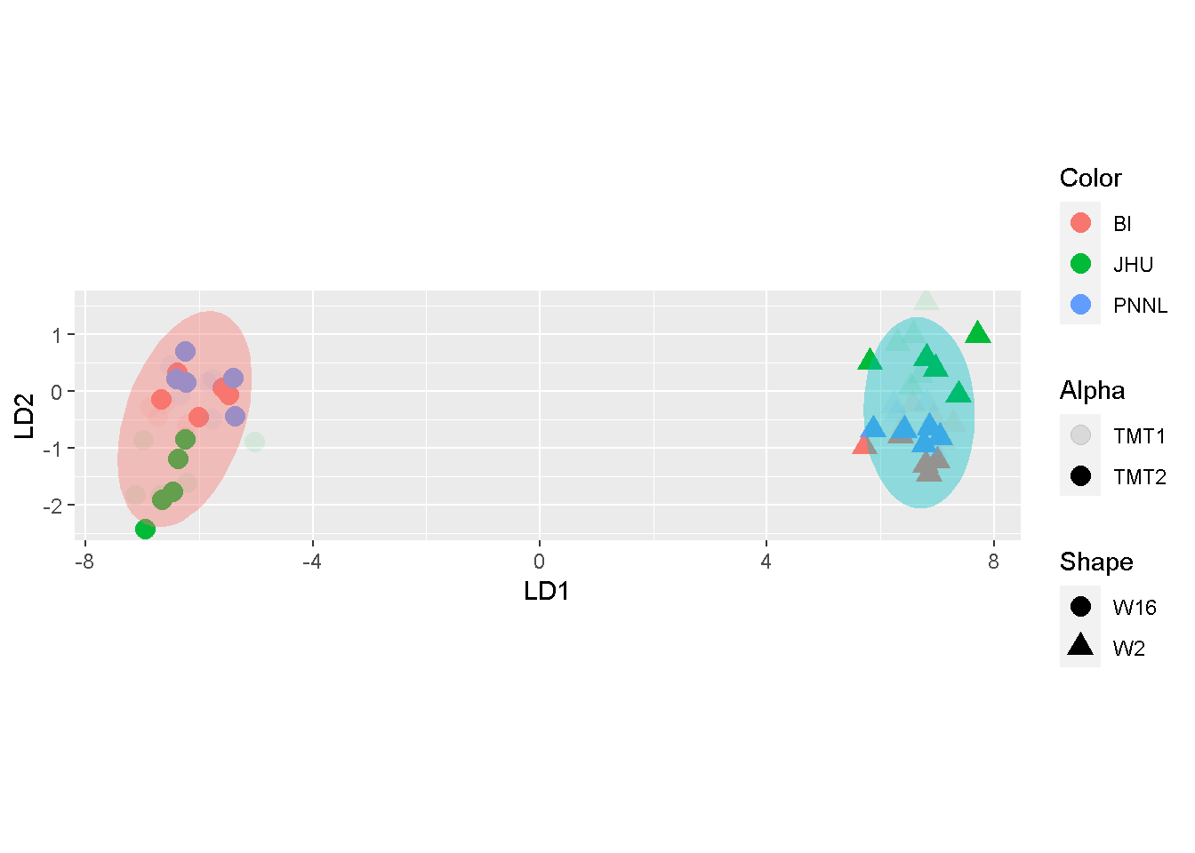 

As mentioned in the beginning of the post, LDA will utilize the response variable, \(\y\). Argument col_group tells prnLDA where to find the values of \(\y\). Unless otherwise specified, it will pick values under the column Group in the metadata file expt_smry.xlsx.

As usual, variable argument statements of filter_ may be applied:

prnLDA(
  col_color = Color,
  col_shape = Shape,
  show_ids = FALSE,
  filter_peps_by = exprs(prot_n_pep >= 5),
  filename = "prns_rowfil.png",
)

More examples are available in help documents via ?prnLDA or pepLDA.

A toy example

We already have PCA. Why do we need LDA? Eqn (1) tells us that PCA decomposes the covariance (or correlation) matrix of the original data whereas eqn (2) shows that LDA breaks the data down by their “separatedness” (ANOVA or MANOVA).³ So, how may we visualize graphically the difference?

In quest of understanding LDA and its properties for a non statistician or mathematician like me, I made up a toy argument that allows the folding of \(p\)-number features (proteins or peptides) under each sample.

What would we get if we split the \(p\)-number proteins equally into two subsets? From the PCA plots shown below, samples were separated by their biological subtypes of W2 and W16 (red and blue ellipses). In addition, they were each well separated by the 2-fold split.

library(ggplot2)

pca <- prnPCA(
  folds = 2,
  col_group = Group,
  col_color = Color,
  col_shape = Shape,
  show_ids = FALSE,
  filename = k2.png,
)

ggplot(pca$pca, aes(PC1, PC2)) +
  geom_point(aes(colour = Color, shape = Shape, alpha = Alpha), 
             size = 4, stroke = 0.02) + 
  stat_ellipse(aes(fill = Shape), geom = "polygon", alpha = .4) + 
  guides(fill = FALSE) + 
  labs(title = "PCA", x = "PC1", y = "PC2") +
  coord_fixed()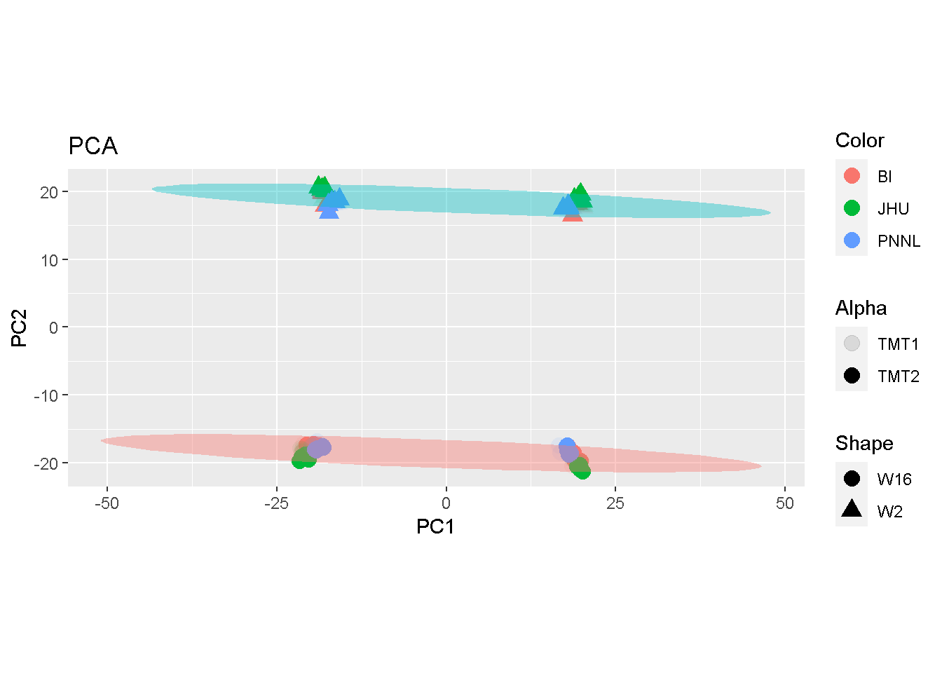 

Similar observation can be found with MDS:

mds <- prnMDS(
  folds = 2,
  col_group = Group,
  col_color = Color,
  col_shape = Shape,
  show_ids = FALSE,
  filename = k2.png,
)

ggplot(mds, aes(Coordinate.1, Coordinate.2)) +
  geom_point(aes(colour = Color, shape = Shape, alpha = Alpha), 
             size = 4, stroke = 0.02) + 
  stat_ellipse(aes(fill = Shape), geom = "polygon", alpha = .4) + 
  guides(fill = FALSE) + 
  labs(title = "MDS", x = "Coordinate 1", y = "Coordinate 2") +
  coord_fixed()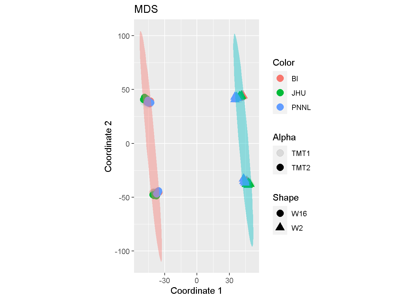 

By contrast, samples were primarily separated by W2 and W16 in LDA. the toy split mostly duplicates the sample-representing dots around the same area, without additional stratification by the split.

lda <- prnLDA(
  folds = 2,
  col_group = Group,
  col_color = Color,
  col_shape = Shape,
  show_ids = FALSE,
  filename = k2.png,
)

ggplot(lda$x, aes(LD1, LD2)) +
  geom_point(aes(colour = Color, shape = Shape, alpha = Alpha), 
             size = 4, stroke = 0.02) + 
  stat_ellipse(aes(fill = Shape), geom = "polygon", alpha = .4) + 
  guides(fill = FALSE) + 
  labs(title = "LDA", x = "LD1", y = "LD2") +
  coord_fixed()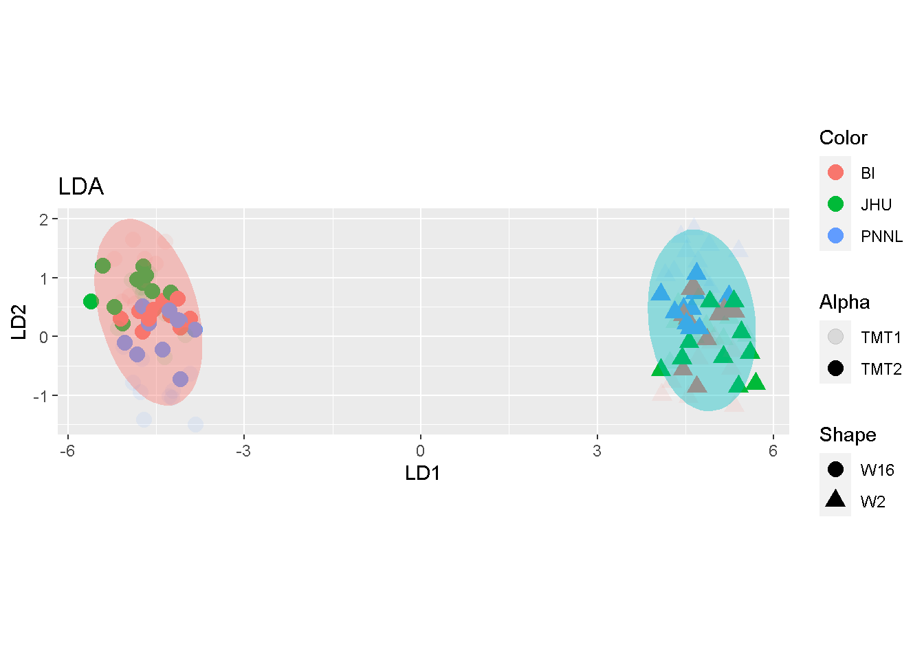 

The comparison seems to suggest that both MDS and PCA may accentuate batch effects whereas LDA articulates mostly the biological difference.

References

Gareth James, Trevor Hastie, Daniela Witten. 2013. An Introduction to Statistical Learning with Applications in R (Print 2015). https://github.com/LamaHamadeh/DS-ML-Books/blob/master/An%20Introduction%20to%20Statistical%20Learning%20-%20Gareth%20James.pdf.
Trevor Hastie, Jerome Friedman, Robert Tibshirani. 2009. The Elements of Statistical Learning: Data Mining, Inference, and Prediction (Print 12th, 2017). https://github.com/tpn/pdfs/blob/master/The%20Elements%20of%20Statistical%20Learning%20-%20Data%20Mining%2C%20Inference%20and%20Prediction%20-%202nd%20Edition%20(ESLII_print4).pdf.
\(\pone\) can be any length here. The division by \(\left \| \pone \right \|^{2}\) to both the numerator and the denominator will cancel out.↩︎
If not, need execution of the
Data normalizationin https://proteoq.netlify.app/post/how-do-i-run-proteoq/. Details available from?load_exptsunder R.↩︎https://stats.stackexchange.com/questions/48786/algebra-of-lda-fisher-discrimination-power-of-a-variable-and-linear-discriminan/48859#48859↩︎
Qiang Zhang
Instructor of Medicine
My research interests include mass spectrometry-based proteomics and automation in data analysis.